Second-order optimization methods

Second-order methods play a crucial role in numerical optimization. Recently, new optimization algorithms, such as Sophia, have emerged in the field of machine learning that make use of the Hessian (the second-order information) or its approximations to achieve better local minima and faster convergence. In this article, our focus will be on unconstrained optimization, where we’ll explore how the Hessian can be a valuable tool.
Theoretical basics
Consider a generic optimization problem
\[\underset{\theta}{\text{min}} \ \mathcal{L}(\theta, y, \hat y)\]where \(\theta\) represents the decision variables (which are typically the parameters of a neural network) that we aim to optimize, \(y\) corresponds to the true labels, and \(\hat y\) stands for the predictions made by the model with parameters \(\theta\). As an example, consider a practical scenario where we are solving a regression problem to predict house prices, and we are using the Mean Squared Error (MSE) as our loss function.
An essential principle in numerical optimization is the First Order Necessary Condition (FONC) which states that if \(\theta^\star\) is local minimizer of \(\mathcal L\), then
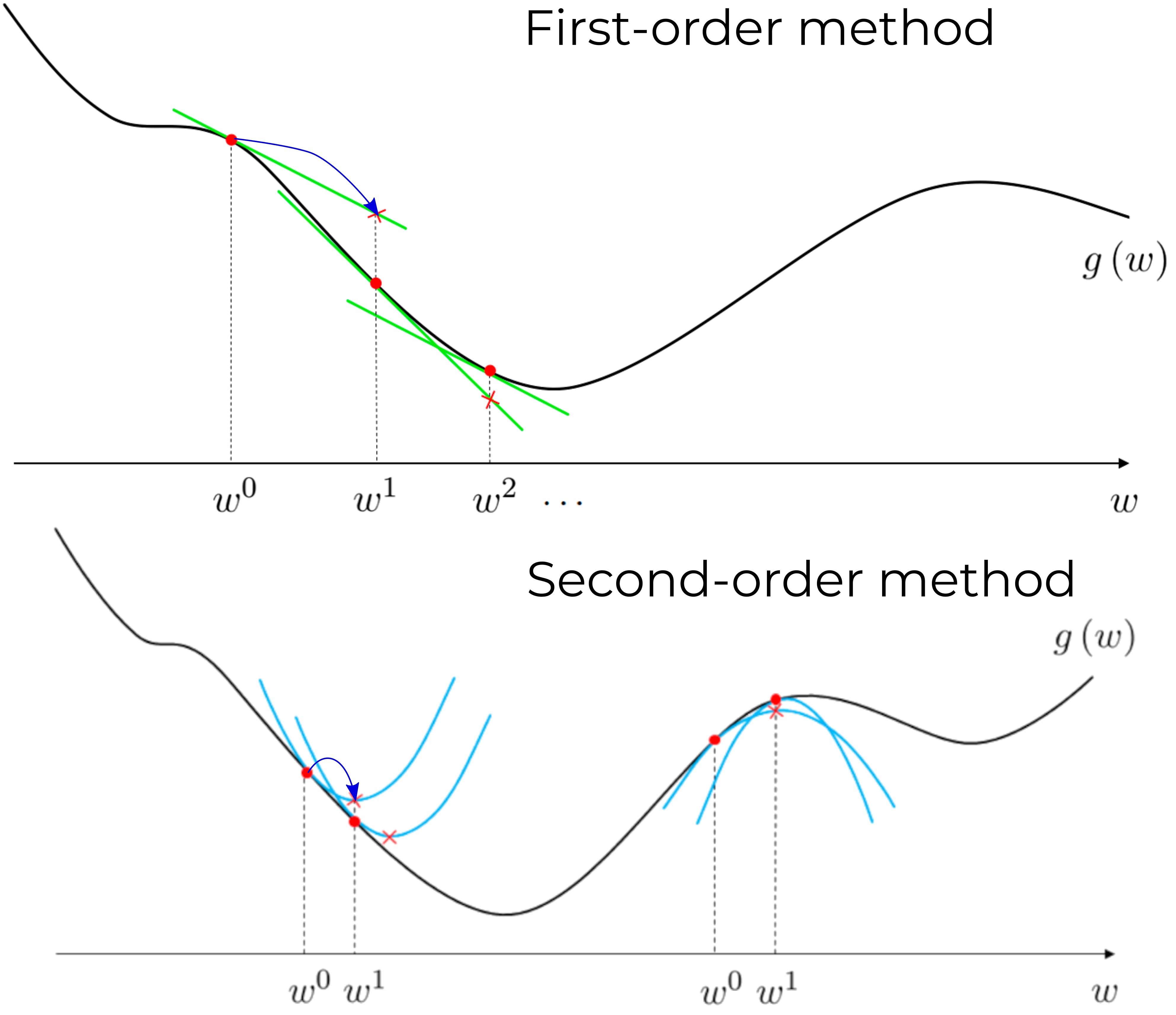
\[\nabla \mathcal L(\theta^\star, \cdot)= 0.\]In simple terms, when we’ve found a solution, our gradient should be zero. If \(\theta\) is scalar, this condition implies that the derivative of the function at the solution should be zero. The point that satisfies \(\nabla_\theta \mathcal L(\cdot)= 0\) is referred to as a stationary point of \(\mathcal L\). Such a point can be either a local minimum, a local maximum, or a saddle point, as depicted in Figure 2.

Since we are specifically interested in finding local minima, we require another condition that ensures our solution \(\theta^\star\) is not a maxima. This condition is known as the Second Order Necessary Condition (SONC), and it states that if \(\theta^\star\) is local minimizer of \(\mathcal L\), then
\[\nabla^2_\theta \mathcal L(\theta^\star,\cdot) \succeq 0.\]Here, \(\nabla^2_\theta \mathcal L(\theta^\star,\cdot)\) represents the second derivative of \(\mathcal{L}\) with respect to \(\theta\) and is referred to as the Hessian. Unfortunately, it’s important to note that saddle points also satisfy the SONC, as illustrated in Figure 1. To guarantee that our solution is indeed a local minimum, we need an even stronger condition known as the Second Order Sufficient Condition (SOSC): \(\nabla^2_\theta \mathcal L(\theta^\star,\cdot) \succ 0\). Now that we have covered the fundamental theory, let’s explore algorithms that leverage second-order information for optimizing our parameters \(\theta\).
Exact Newton’s method
Newton’s method (Newton-Raphson method) is a technique primarily used for solving root-finding problems. In fact, the First Order Necessary Condition can be framed as a root-finding problem: we need to find parameters \(\theta^\star\) that make the gradient of the loss function equal to zero. To achieve this, we can apply Newton’s method, which leverages the Taylor series expansion of \(\nabla \mathcal{L}\):
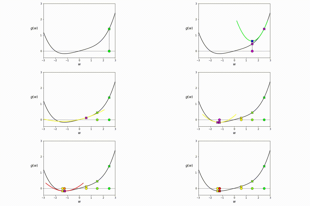
\[\begin{align*} \nabla \mathcal L(\theta_k) + \frac{\partial }{\partial \theta} (\nabla \mathcal L(\theta_k))(\theta - \theta_k) = 0, \\ \theta_{k+1} = \theta_k - \nabla^2 \mathcal L(\theta_k)^{-1} \nabla \mathcal L(\theta_k). \end{align*}\]When starting from the loss function \(\mathcal{L}\), we expand it into a Taylor series, considering terms up to the second order. In simpler terms, Newton’s method locally approximates the loss with a quadratic function, computes the minimum of this quadratic approximation, and iteratively refines it until convergence, as illustrated in the gif below.

Newton Type Methods
We saw that Newton’s method relies on the Hessian for parameter updates. However, computing the Hessian can be computationally demanding. As a result, researchers have devised various methods to approximate the Hessian and avoid its explicit computation. Generally, these methods follow a common structure:
\[\theta_{k+1} = \theta_k - B_k^{-1}\nabla \mathcal L(\theta_k)\]Levenberg-Marquardt
Levenberg-Marquardt (LM) is a widely-used method for solving nonlinear least-squares problems, frequently applied in Simultaneous Localization and Mapping (SLAM) for both camera and LiDAR-based. The core concept behind LM involves locally approximating the loss function with a quadratic model. Consider the following least-squares loss function:
\[\mathcal{L} = \frac{1}{2}||l( \theta, y, \hat y)||_2^2 + \frac{1}{2} \lambda ||\theta||_2^2\]Let’s expand \(l( \theta, y, \hat y)\) using a Taylor series and retain only the first two terms:
\[l \approx l(\theta_k) + \nabla l(\theta_k)^T (\theta - \theta_k) + \mathrm{h.o.t.}\]Substituting this back into the loss function yields:
\[\begin{align} \mathcal{L} &= \frac{1}{2}\big(l - \nabla l (\theta - \theta_k)\big)^T\big(l - \nabla l (\theta - \theta_k)\big) + \frac{1}{2}\lambda\theta^T \mathbb{I} \theta \\ &=\frac{1}{2}\big(l^Tl + 2l^T \nabla l (\theta - \theta_k) + (\theta - \theta_k)^T \nabla l^T \nabla l (\theta - \theta_k)\big) + \frac{1}{2}\lambda\theta^T \mathbb{I} \theta \\ & = \frac{1}{2} l^T l + l^T \nabla l(\theta - \theta_k) + \frac{1}{2}(\theta - \theta_k)\underbrace{(\nabla l^T \nabla l + \lambda \mathbb{I})}_{B} (\theta - \theta_k) \end{align}\]From equation (3), it’s evident that the LM approximation of the Hessian matrix is given by \(B_k = \nabla l^T \nabla l + \lambda \mathbb{I}\). The regularization term \(\lambda \mathbb{I}\) ensures that \(B\) is always invertible, even when \(\nabla l^T \nabla l\) is singular. Therefore, one iteration of the LM method is expressed as:
\[\theta_{k+1} = \theta_k - \left(\nabla l^T \nabla l + \lambda \mathbb{I}\right)^{-1} \nabla \mathcal L(\theta_k)\]Gradient Method
Gradient Method (GM) or steepest descent method is one of the most widely used optimization techniques in machine learning. This method approximates the Hessian matrix with the identity matrix, weighted by the inverse of the learning rate \(\alpha\): \(B = \frac{1}{\alpha}\mathbb{I}\). Consequently, the optimization steps can be expressed as:
\[\theta_{k+1} = \theta_k - \alpha \nabla \mathcal L(\theta_k)\]Quasi-Newton Methods
Quasi-Newton Methods (QNM) approximate the Hessian matrix \(B_{k+1}\) based on the knowledge of \(B_k\), \(\nabla \mathcal L(\theta_k)\) and \(\nabla \mathcal L(\theta_{k+1})\). Among the various methods for determining the update to the Hessian matrix \(B_{k+1}\), one widely used and successful approach is the Broyden–Fletcher–Goldfarb–Shanno (BFGS) algorithm. In the BFGS algorithm, the curvature of the function is approximated using finite differences. In simpler terms, we choose the matrix \(B_{k+1}\) in a way that satisfies the secant condition:
\[B_{k+1} \left(\theta_{k+1} - \theta_k \right) = \nabla \mathcal L(\theta_{k+1}) - \nabla \mathcal L(\theta_{k}).\]The rationale for selecting this condition is that the Hessian \(\nabla^2 \mathcal L(\theta_k)\) satisfies it as \(\theta_{k+1}\) approaches \(\theta_{k}\). Since multiple matrices can satisfy the secant condition, we can reasonably assume that \(B_{k+1}\) and \(B_k\) should be close to each other. Therefore, we choose \(B_{k+1}\) as the matrix closest to the previous Hessian approximation \(B_k\) among all matrices that satisfy the secant condition. To measure the proximity between \(B_{k}\) and \(B_{k+1}\), we can employ the concept of differential entropy between random variables with zero-mean Gaussian distributions \(\mathcal{N}(0, B_k)\) and \(\mathcal{N}(0, Z)\) which can be formulated as a semidefinite program. This program (optimization problem) has an analytical solution in the form
\[\begin{align*} B_{k+1} &= B_k - \frac{B_k s s^T B_k}{s^T B_k s} + \frac{y y^T}{s^T y}, \\ s &= \theta_{k+1} - \theta_k, \\ y &=\nabla \mathcal L(\theta_{k+1}) - \nabla \mathcal L(\theta_{k}). \end{align*}\]Recall that the Hessian matrix is often dense and has dimensions \(n_\theta \times n_\theta\), where \(n_\theta\) represents the number of parameters we intend to optimize. Consequently, storing this matrix in memory can be memory-intensive. To address this issue, a variant of BFGS known as Limited-memory BFGS (L-BFGS) was developed. L-BFGS overcomes the memory challenge by having a linear memory requirement. In contrast to BFGS, which stores the Hessian approximation matrix \(B_k\), L-BFGS maintains a history of the previous \(m\) updates of both the parameters \(\theta\) and the gradient \(\nabla \mathcal L(\theta)\). This approach allows L-BFGS to implicitly represent the Hessian approximation using only a few vectors.
Scalable second-order method for deep learning
Second-order Clipped Stochastic Optimization (Sophia) goes one step further in reducing computational overhead by approximating the Hessian using a diagonal matrix. Additionally, it incorporates a clipping mechanism to control the maximum update size. This feature is essential because rapid changes in the landscape of the loss function could make the second-order information unreliable.

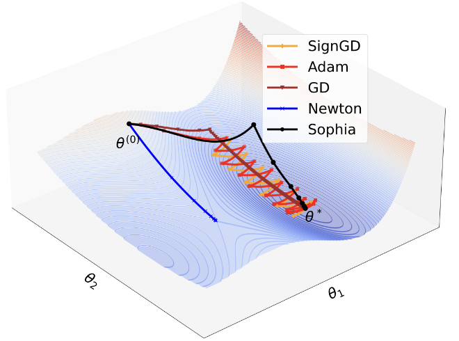
Concretely, Sophia estimates the diagonal entries of the Hessian of the loss using a mini-batch of examples every \(k\) steps. At each step, Sophia updates the parameters using an exponential moving average (EMA) of the gradient divided by the EMA of the diagonal Hessian estimate, which is then clipped by a scalar. Experiments on training LLM on GPT-2 dataset show that Sophia is twice as fast as the AdamW (Figure 4).

Case study
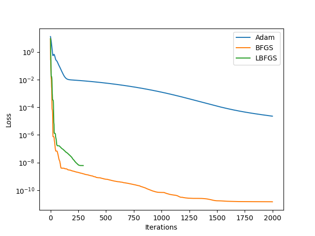
The test case was adopted from the Study on Optimizers, which utilized a four-layer network consisting of 20 neurons per layer, all employing the hyperbolic tangent (tanh) activation function. This network was trained to fit the dataset \(\mathcal{D} = \{x_i, \sin(x_i) \}_{i=1}^{100}\), where \(x_i\) was sampled from a uniform distribution \(\mathcal{U}(0,1)\). The mean squared error (MSE) served as the loss function during training. The results on training using different optimizers are shown in the Figure 5.

The results from this toy example and findings from the Sophia paper clearly demonstrate that Newton-type optimization methods are significantly faster and yield lower loss values. This indicates the potential usefulness of second-order methods for training neural networks.
Useful resources
- Machine Learning Refined is an excellent book with jupyter notebooks that visually explains zero-, first- and second-order optimization methods.
- Patterns, Predictions, and Actions is another excellent book that explains the basics of the second-order methods.