Figure 1. A vector field of a damped pendulum

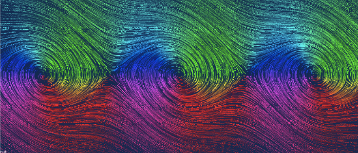
Differential equations serve as the natural language of physics and nature. Remember back in school when you were taught Newton’s Second Law of Motion: $F = ma$? The acceleration $a$, represents the second derivative of the position $x$. Consequently, we have $F = m \ddot x$, which is a second-order ordinary differential equation (ODE). Differential equations find wide application in various fields, including biology, economics, and sociology, as they can effectively model numerous phenomena.

On the other hand, machine learning and other data-driven methods have demonstrated their ability to successfully predict behaviors of complex systems. The question arises: How can we combine machine learning with differential equations to construct more robust models for understanding and representing natural phenomena?

Ordinary differential equations recap

In general, a differential equation can be expressed in the form: $$ \frac{d}{dt}z(t) := \dot z(t) = f\left(t,z(t), \theta\right) $$ Here, $z(t)$ represents the state, $f(\cdot)$ denotes the vector field, $t$ corresponds to time, and $\theta$ represents the parameters. An example of the vector field is shown in the Figure 1. Essentially, an ODE models the rate of change of variables. For instance, consider the differential equations governing a simple pendulum shown in the figure 2:

Figure 2. A drawing of a simple pendulum

\[\dot z(t) = \begin{bmatrix} z_2(t)\\ -\frac{g}{L} \sin(z_1(t)) \end{bmatrix}\]

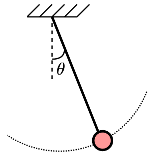
In this case, $z_1(t):=\theta$ denotes the angle of the pendulum, $z_2(t):=\dot \theta$ represents the angular velocity, $g$ denotes the gravitational constant, and $L$ stands for the length of the pendulum. Intuitively, pendulum ODE describes how the angle and angular velocities change.

When working with differential equations, it is crucial to specify the initial state. Without knowing the initial condition $z(t_0)$, it becomes impossible to solve the differential equation aka to integrate it. It is worth noting that the majority of real-world differential equations do not have analytical solutions. However, numerical methods have been developed to approximate solutions at discrete points. These methods involve integrating the equation over a given interval

\[z(t_1) = z(t_0) + \int_{t_0}^{t_1} f(t, z(t), \theta)\ dt = \text{ODESolve}(z(t_0), f, \theta, t_0, t_1)\]

In the following subsections, we will explore two simple methods that provide a glimpse into solving ODEs using numerical techniques and quickly discuss advanced methods.

Euler Methods

One of the simplest methods for numerical integration is Euler's method. It is derived from the basic definition of the tangential approximation of the gradient at a point $$ \frac{dz(t)}{dt} \approx \frac{z(t+\Delta t) - z(t)}{\Delta t} $$ where $\Delta t$ is a fixed step-size. By rearranging this expression, we obtain the final form of the Euler integrator

Figure 3. Visualization of the Euler method [1]

\[z(t+\Delta t) = z(t) + \Delta t \frac{dz(t)}{dt} = z(t) + \Delta t \ f\big(t, z(t), \theta \big)\]

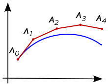
To integrate an ODE using Euler method, we begin with an initial time $t_0$, initial state $z(t_0)$ and a step-size $\Delta t$. We then iteratively compute the trajectory of the ODE until we reach final time $t_N := t_0 + N \Delta t$

\[\begin{align*} z(t_1) = z(t_0) + \Delta t\ f(t_0, z(t_0), \theta),\quad t_1 = t_0 + \Delta t \\ z(t_2) = z(t_1) + \Delta t\ f(t_1, z(t_1), \theta),\quad t_2 = t_1 + \Delta t \\ \dots \\ z(t_N) = z(t_{N-1}) + \Delta t\ f(t_{N-1}, z(t_{N-1}), \theta),\quad t_N = t_{N-1} + \Delta t \end{align*}\]

One intuition behind the Euler method is that we are evolving the trajectories by iteratively taking small steps in the direction of the slope.

Runge-Kutta Methods

Despite being easy to understand and implement, the Euler method is often not used in practice due to its low accuracy. Instead, a more commonly employed method that strikes a balance between computational efficiency and accuracy is the fourth-order Runge-Kutta (RK4) method. This method involves computing the state at the next time step by taking four intermediate steps

\[z(t + \Delta t) = z(t) + \frac{1}{6} \Delta t(k_1 + k_2 + k_3 + k_4)\]

where

$$ \begin{align*} k_1 = f(t, z(t), \theta) \\ k_2 = f(t + \frac{\Delta t}{2}, z(t) + \Delta t\ \frac{k_1}{2}, \theta) \\ k_3 = f(t + \frac{\Delta t}{2}, z(t) + \Delta t\ \frac{k_2}{2}, \theta) \\ k_4 = f(t + \Delta t, z(t) + \Delta t\ k_3, \theta) \end{align*} $$ Derivation of the RK4 equations is out of scope of this article. I will only quickly mention that it is based on the Taylor expansion of both $z(t + \Delta t)$ and $f(t+\Delta t, z + \Delta z)$.

Integrating an ODE with RK4 is similar to the Euler method and to any other method with fixed step size: define initial time $t_0$ initial state $z(t_0)$ step size $\Delta t$ and the number of steps $N$ then in a for loop we iteratively compute the state $z(t)$ at discrete moments of time $t_0, t+\Delta t, \dots , t+ N \Delta t$.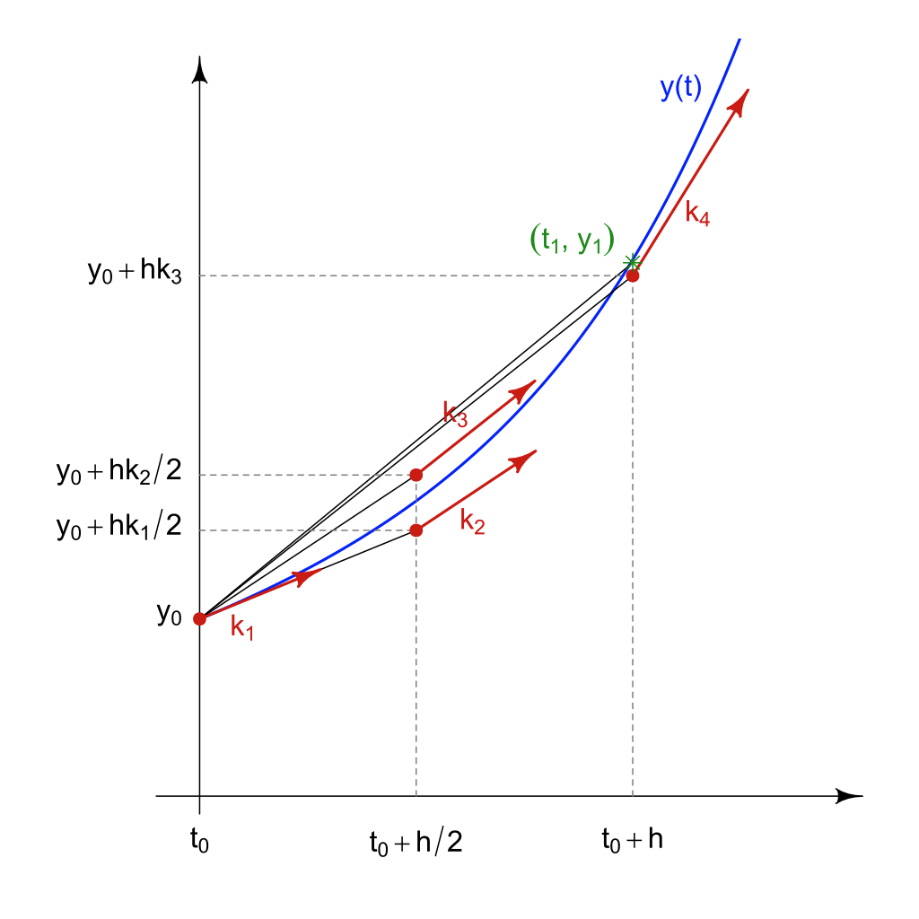

Figure 4. Visualization of the RK4 method [2]

Variable step-size methods

To achieve greater accuracy than RK4, we can utilize variable step solvers. These solvers dynamically adjust the step-size to meet specified absolute and relative tolerances. One prominent example of such integrators is the Dormand-Prince method (DP45). The DP45 method determines the appropriate step-size by estimating the integration error, which is computed by comparing the results of the 5th and 4th order Runge-Kutta methods. However, a trade-off for this increased accuracy is the additional computational time required, as the number of steps needed for ODE integration cannot be predetermined.

Neural Differential equations

Now that we have a solid understanding of what ODEs are and how to solve them, we can explore the process of obtaining the ODE itself. While it may be relatively straightforward to derive the vector field $f$ for simple systems like a pendulum, tackling complex systems such as robots or virus spread rates requires extensive domain knowledge. Furthermore, even if we manage to obtain the vector field, ensuring the accuracy of the parameters $\theta$ within that vector field can be challenging. This is due to the numerous assumptions and simplifications made when formulating physical laws (consider the ideal gas assumption, for instance).

If we are provided with input-output data, we can employ a function approximator to estimate the underlying vector field $f$. One popular choice for this approximator is a neural network, leading to the concept of Neural Ordinary Differential Equations (Neural ODEs):

\[\dot z(t) = NN\big(t, z(t), \theta_{NN}\big)\]

Comparison to Resnets

When we apply the Euler method to integrate a Neural ODE, we obtain an equation that closely resembles a ResNet

\[z(t+\Delta t) = z(t) + \Delta t \ NN(t, z(t), \theta_{NN})\]

with the only difference being the scaling coefficient $\Delta t$. If we allow the neural network $NN(\cdot)$ to incorporate the $\Delta t$ parameter $\tilde{NN}(\cdot) = \Delta t\ NN(\cdot)$, the Neural ODE integrated with the Euler method effectively becomes a ResNet.

\[z(t+\Delta t) = z(t) +\tilde{NN}(t, z(t), \theta_{NN})\]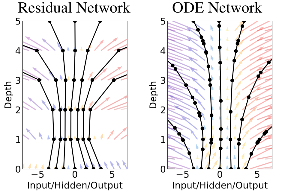

Figure 5. Comparison between ResNet and an ODE Network [3]

Earlier we learned that the Euler integrator is outperformed by other integration methods like the RK4 or variable step integrators. Therefore, utilizing Neural ODEs with these improved integrators can lead to more accurate and reliable models than ResNets. Furthermore, Neural ODEs can be viewed as infinite-dimensional networks: ResNets provide a solution at a discrete points and have low accuracy, but Neural ODEs with the adaptive step-size has higher accuracy and smooth vector field as shown in the Figure 4. If we want to get the same accuracy with the ResNets we need to make them very deep.

Training and gradients

If you’re already wondering about training these beasts called Neural ODEs and the intimidating concept of viewing them as infinite depth ResNets, fear not! Computing gradients for Neural ODEs is actually quite efficient and requires minimal memory.

Let’s say we have a dataset $\mathcal{D} = \{x_i, y_i\}$ where $x$ represents the input and $y$ represents the target. For example, let $x$ be the angle and angular velocities of the pendulum and $y$ be the same quantities but after 1 second. Our goal is to train a Neural ODE to predict the target using a loss function $\mathcal{L}(\hat y, y)$. We can express the predicted output $\hat y_i$ as:

\[\hat y_i := z(t_1) = \text{ODESolve}(z(t_0), NN, \theta_{NN}, t_0, t_1)\]

Here, $\text{ODESolve}$ can be any integrator, $y(t_0) := x_i$ represents the initial state of our Neural ODE, and $t_0$ and $t_1$ are the initial and final integration times, respectively. When using variable step integrators, we may perform numerous intermediate computations, resulting in a large computational graph. Consequently, performing backpropagation through this graph can be computationally expensive and slow.

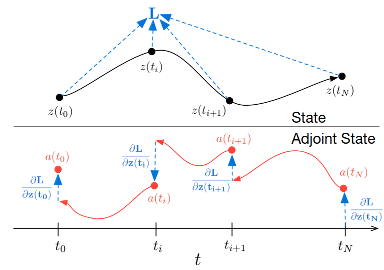
Figure 6. Backpropagation of a Neurtal ODE [3]

However, it turns out that obtaining the gradients of $\hat y_i$ with respect to the states $z(t)$, parameters $\theta_{NN}$, and time $t$ is surprisingly straightforward. We simply need to integrate an additional ODE (backward in time) that provides all these gradients. This powerful technique is known as the adjoint method. While the derivations can be somewhat involved, if you want to dive into math here are two excellent sources: the method of Lagrange multipliers and the method described in the original paper.

In this article as an example we considered regression problem, but Neural ODE can also be used for classification. For those task Neural ODE has to make different classes linearly separable at the end of the integration.

Pros and cons

According to the seminal paper, Neural ODEs offer several advantages over deep ResNets. They allow for more memory-efficient training and require fewer parameters. Additionally, the backpropagation process is more computationally efficient with Neural ODEs.

Neural ODEs are particularly well-suited for time series data, especially when the dataset is irregularly sampled, which is often the case. When dealing with non-uniform, classical methods like RNNs require special treatment. In contrast, Neural ODEs naturally handle non-uniform data by adapting the time grid of the integrator.

From a personal perspective, training Neural ODEs is slower compared to training RNNs. In case of uniform data, use RNNs for their efficiency.

Software

Nowadays there are many libraries that facilitate the training of Neural ODEs. If you prefer working with PyTorch, use either torchdiffeq or torchdyn. These libraries provide comprehensive functionalities for building and training Neural ODE models within the PyTorch framework. On the other hand, if you opt for JAX, I highly recommend diffrax.

Resources

[1] Wikipedia article on Euler method

[2] Wikipedia article on Runge-Kutta methods

[3] Seminal paper on neural ordinary differential equations