Imagine you’re trying to predict the behavior of a complex system, like a weather pattern, a financial market or a robot. In an ideal world, you would have access to all of the relevant data needed to accurately model the system (full state measurement). However, in reality, we rarely have access to a full state only to partial observations (outputs) which might be a subset of states or some nonlinear transformation of states. This presents a challenge for machine learning algorithms that rely on full state measurement.

In this post, we’ll explore several methods for learning system dynamics from partial observations. We’ll discuss why this problem is important, and why it’s relevant to real-world applications like predicting weather, stock prices or robot behavior. By the end of this post, you’ll have a better understanding of the challenges involved in learning system dynamics from partial observations, and the methods that are currently being used to tackle this problem.

Problem formulation

To understand how we can learn system dynamics from partial observations, we need to define the problem more precisely. Let’s start with the ground truth nonlinear discrete dynamics, which can be defined by the following difference equation:

\[x_{k+1} = F\big(x_k, u_k, \theta_{r}\big)\]

where \(x_k = x(t_k)\) is the vector of states of the system at time \(t_k\), \(u_k\) is the vector of external inputs and \(\theta_r\) is the vector of true parameters of the system. Let \(y_k\) represent noisy observations (measurements) of the system

\[y_k = H\big(x_k\big) + \nu_k\]

where \(H(x_k)\) is the state-to-observation map and \(\nu_k\) is a noise. As an example, imagine we need to learn a robot dynamics shown in Figure 1. The states of the robot are joint positions and velocities. But assume that the data are external inputs (joint torques) and positions of some keypoints measured using a camera while the robot is moving.

Figure 1. Robot as an example of partially observable system

Given these noisy measurements, we would like to learn an approximation of the original system dynamics \(\hat z_{k+1} = \hat F(\hat z_k, u_k, \theta_a)\) with \(\hat F(\cdot)\) being the approximation of the original state transition map \(F(\cdot)\) and \(\theta_a\) being the parameters of the approximate transition map. If we know the dimension of the original state \(x\), then we can choose \(z\) to be of the same size. Otherwise — if we don’t know the dimension or want to find a lower dimensional approximation of the map \(F(\cdot)\) — we can choose the dimension of \(z\) arbitrarily to a degree that it can accurately predict outputs \(y.\)

Figure 2. Working principle of an RNN

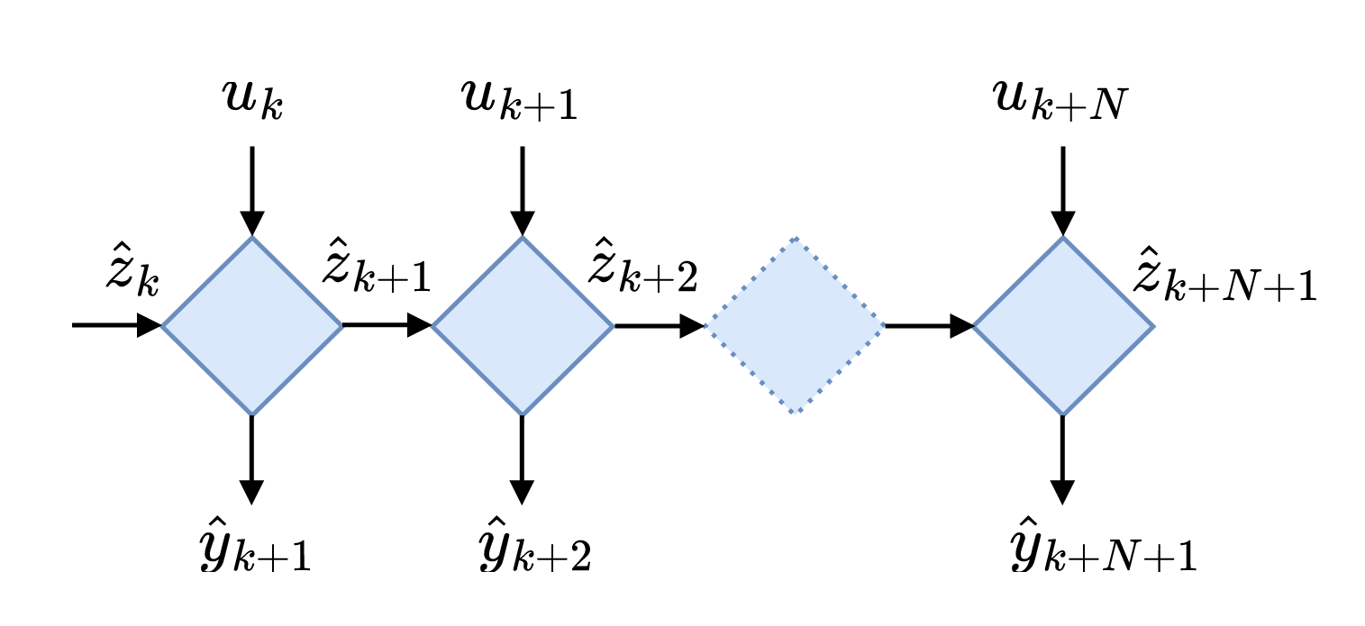
For the sake of simplicity, lets use recurrent neural networks (RNNs) for approximating the dynamics. Figure 2 shows schematically the working principle of the vanilla RNN, where each rhomb is an RNN block. In a nutshell, RNN takes an input \(u_k\) and state \(\hat z_k\) and spits out the next state \(\hat z_{k+1}\). Mathematically spaeking, vanilla RNN propagates dynamics by

\[\hat z_{k+1} = \tanh(W_{\hat z} \hat z_k + W_u u_k + b).\]

To sum up, we are interested in learning the model of a complex dynamical system from partial observations. The model should accurately predict \(N\) next states/observations of the system: \(z_{k+1}\), \(z_{k+2}\), \(\dots\), \(z_{k+N+1}\). In essence, the problem we trying to solve boils down to finding an initial state \(z_0\) that will be used by RNN to propagate the dynamics and state-to-observation transformation \(\hat H(\cdot)\). Now, lets dive into several methods that have been proposed to solve this problem.

Autoencoders

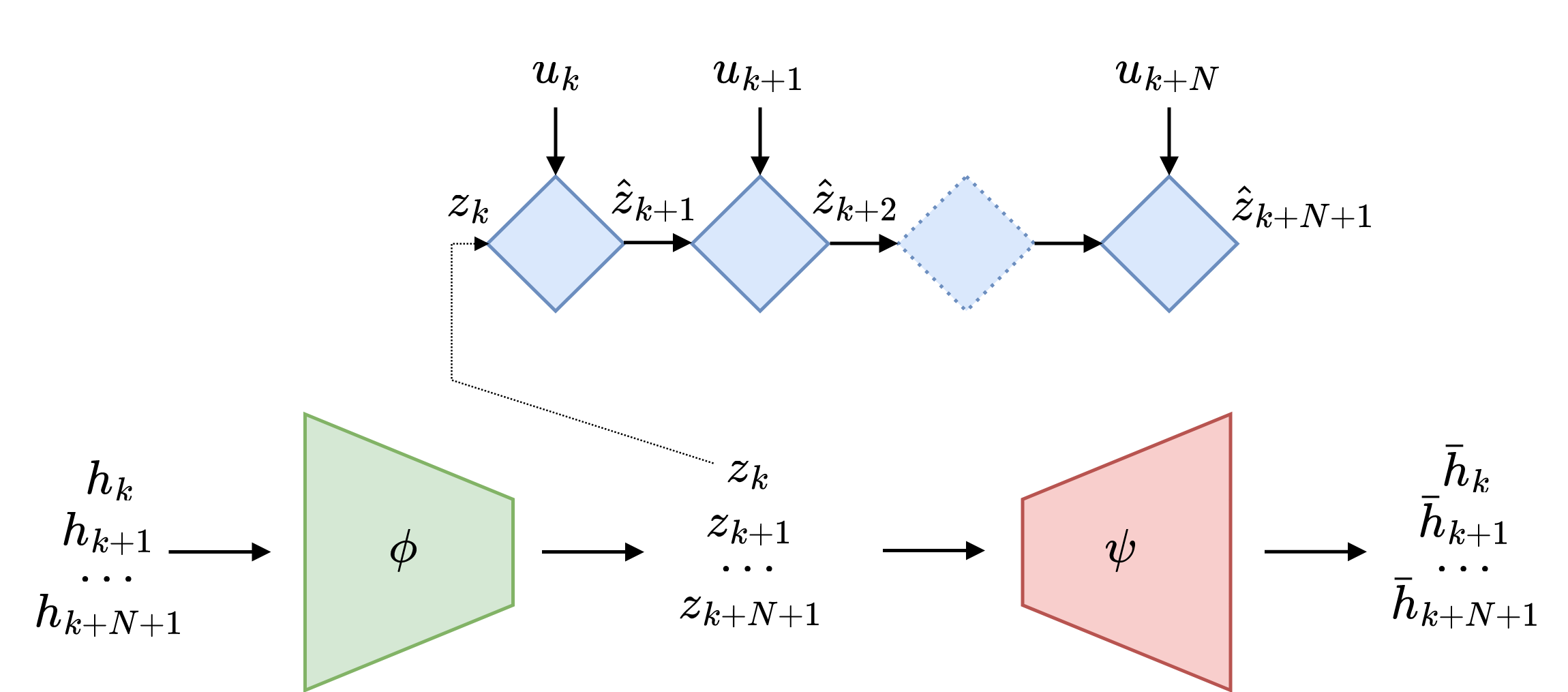
A common approach in machine learning for solving such problems is autoencoders. Here our input feature vector \(h\) for the encoder is a sequence of output and input measurements. For simplicity, let’s choose \(h_k = \left(y_k; u_k\right)\). The encoder—a multilayer perceptron (MLP)—takes the input vector \(h_k\) and outputs the latent state \(z_k = \phi\left(h_k\right)\). Given the latent state and a sequence of inputs \(U = [u_k\ u_{k+1} \dots u_{k+N}]\), the RNN propagates the dynamics and returns a sequence of states \(\hat{z}_{k+1},\ \hat{z}_{k+2},\ \dots,\ \hat{z}_{k+N}\). The decoder—another MLP—takes states and maps them into a sequence of outputs \(\hat{y}_{k+1},\ \hat{y}_{k+2},\ \dots,\ \hat{y}_{k+N}\).

Figure 3. Autoencoder based latent dynamics learning

The loss function of the whole end-to-end learning is a combination of several losses:

encoder-decoder loss which measures how well the enocder-decoder pair work together

\[\mathcal{L}_1= \sum_{k=1}^{N} ||h_k - \psi(\phi(h_k)) ||_2^2\]

state reconstruction loss which measures if encoded latent state matches the dynamics of the system

\[\mathcal{L}_2 = \sum_{j=1}^{N} ||z_{k+j} - \hat z_{k+j}||_2^2\]

Output prediction loss which measures how well the dynamics approximates the true dynamics

\[\mathcal{L}_3 = \sum_{j=1}^N||h_{k+j} - \psi(\hat z_{k+j})||\]

The total loss function is the weighted sum of the individual losses: \(\mathcal{L} = \alpha \mathcal{L}_1 + \beta \mathcal{L}_2 + \gamma \mathcal{L}_3\) . One paper where such an approach has been used in combination with SINDY is link. Check it out for more detail.

RNN Encoders

Another machine learning approach is to use an RNN as an encoder to learn the latent dynamics. In this method, we take a sequence of observation and external input pairs \((y_{k}, u_{k}),\ (y_{k+1}, u_{k+1}),\ \dots, \ (y_{k+M}, u_{k+M})\) and feed it to an RNN backwards in time, where the final state of the RNN is the sought-after state \(z_k\). In a probabilistic setting, the final state of the RNN represents the mean and covariance of the distribution \(z_k \sim \mathcal{N}(\mu_k, \Sigma_k)\). Typically, the RNN encoders state is initialized with a zero vector.

Figure 4. RNN encoder based latent dynamics learning

If you are familiar with sequence-to-sequence modeling, you may recognize the RNN encoder architecture from machine translation. In this context, the RNN encoder provides “context” for the RNN decoder, which generates a translation based on it.

This scheme works well due to the stability of dynamical systems. Stable dynamical systems “forget” their initial state and converge to a stationary point. Therefore, it’s a good idea to choose a relatively large input sequence MM to give it time to converge. RNN encoders have been used extensively in learning latent dynamics with neural ordinary differential equations, for example in this and this papers.

Learning the initial state

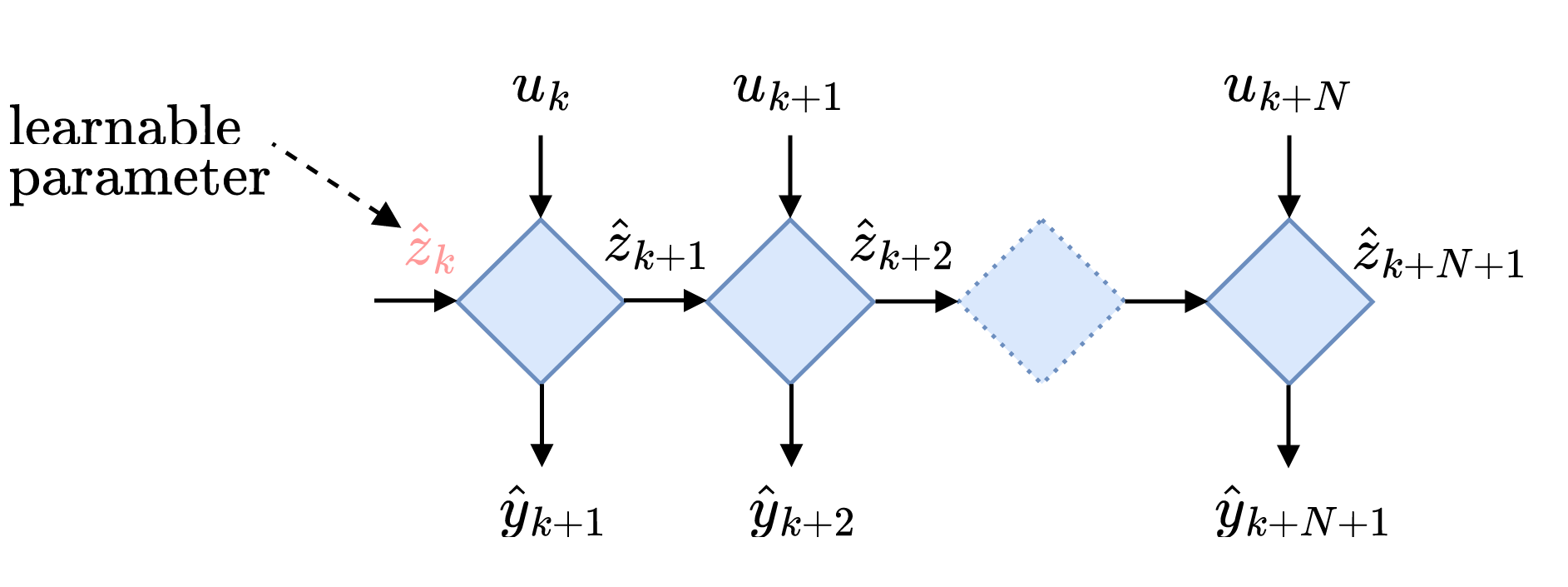
The system identification community has developed its own tools for learning latent dynamics, and one of the simplest methods is to make the initial state an optimization variable and eliminate the need for an encoder. This approach is often used for grey box system identification, where the system structure \(F(x_k, u_k, \theta_r)\) and the state-to-output map \(H(x_k)\) are known but the parameters \(\theta_r\) are not. However, this method can also be used for more generic (black box) model architectures such as RNNs. Nevertheless, making the initial state an optimization variable increases the number of optimization variables, especially when using mini-batch optimization. Therefore, it only makes sense to learn the initial state when trying to predict long horizons and using batch optimization. This method has been used in various works, including the work by my colleague in MECO Andras.

Figure 5. Learning latent state for latent dynamics learning

KKL encoder

The majority of control policies for robots, planes, or chemical plants rely on the latent state to compute the action. Control engineers have developed algorithms called state estimators or observers to infer latent states from partial observations. The most famous among them are the Kalman filter and its variations, such as the extended Kalman filter and the unscented Kalman filter. However, most state estimation algorithms heavily rely on the latent dynamical model of the system. In our setting, using classical state observers would lead to a chicken-and-egg problem: we need to infer the latent state from partial observations to learn the latent dynamical model, but we need the latent dynamical model to do so.

Among the few state estimation algorithms that do not heavily rely on an accurate dynamical model is the Kazantzis-Kravaris Luenberger (KKL) observer. The KKL observer separates the latent dynamics \(z_{k+1} = \hat F(z_k, u_k, \theta_a)\) from the observer dynamics and assumes linear dynamics for the observer, where the state of the KKL observer, denoted by xi, evolves according to the following equation:

\[\xi_{k+1} = D \xi_k + G \begin{bmatrix} y_k \\ u_k \end{bmatrix}\]

where \(D\) is a stable state matrix with eigenvalues \(-1 < \lambda_i < 1\). The stability requirement guarantees that no matter how we initialize \(\xi\), after a sufficiently long time, the observer will converge and “forget” its initial state. The KKL observer is able to separate observer dynamics from latent dynamics because there exists a smooth invertible map \(\mathcal{T}\) that goes from our latent state \(z\) to the observer state \(\xi\) and back. Unfortunately, there is no ready-to-use recipe for finding such a map. In practice, we can think of the map \(\mathcal{T}\) and its inverse \(\mathcal{T}^*\) as an autoencoder that is jointly learned together with the latent dynamics. The difference between the purely autoencoder approach and the KKL observer approach is that the input of the encoder is the KKL observer state instead of a sequence of observations and external inputs (as shown in Figure 6). Check out this paper, if you want to learn more about KKL encoder method.

Figure 6. KKL encoder based latent dynamics learning

Conclusions

In real life, we often have to train models to predict the behavior of complex dynamic systems based on partial observations. To train a model with hidden variables, we need to somehow estimate/reconstruct the initial hidden state, and then propagate the hidden state using the chosen architecture and sequence of (external) inputs. There are various methods for estimating the initial hidden state. Perhaps the simplest method is to make the initial state an optimization variable. This method has one major drawback: depending on the type of learning (batch vs mini-batch) and the duration of the dynamics propagation, the number of optimization variables can grow significantly.

The most common method is probably the autoencoder, where the encoder takes a sequence of partial observations and external inputs as input and returns the hidden state. The decoder, in turn, takes the hidden state as input and tries to reconstruct the encoder input. The next two methods - RNN and KKL encoders - are dynamic: they take a partial observation and an external input as input, propagate the dynamics back in time to find the initial hidden state.

In this article, it is shown that the difference between different approaches is not very significant for modeling the hidden dynamics of an exoskeleton. Therefore, in practice, I would first implement an autoencoder. If the model quality is unsatisfactory, I would switch to dynamic encoders.