The robotics community has shown significant interest in deformable object manipulation in recent years, with workshops hosted at ICRA and IROS in 2022. Both model-based and model-free approaches rely on accurate simulators. The finite element method (FEM), a powerful tool from continuum mechanics, can be computationally expensive for control. The rigid finite element method (RFEM) is a simpler and faster approach that can leverage existing rigid-body dynamics tools.

While not a new method, the RFEM — also known as the extended-flexible joint method or pseudo-rigid body method — remains a valuable modeling technique in robotics. This post explores its basic principles, limitations, and trade-offs, and provides a practical tutorial on simulating simple deformable linear object in Python using the Pinocchio library.

Whether you’re a seasoned researcher or new to the field, this post offers valuable insights and practical guidance on using the RFEM to model deformable linear objects.

Basics of the RFEM

RFEM is a pretty straightforward way to study deformable objects by dividing them into smaller parts called rigid finite elements (rfes) and connecting them with spring-damping elements (sde). The technique uses generalised coordinates based on the elements’ displacements to describe the position of the system.

To make things clearer, let’s consider a simple example of a cylindrical rod attached to a motor, as you an see in Figure 1. This setup can be thought of as an elastic pendulum or a deformable linear object that is manipulated by a robot arm. For now, we will only talk about dominant bending flexibility and describe the displacements of each rfe relative to the preceding element.

The RFEM discretizes in two stages:

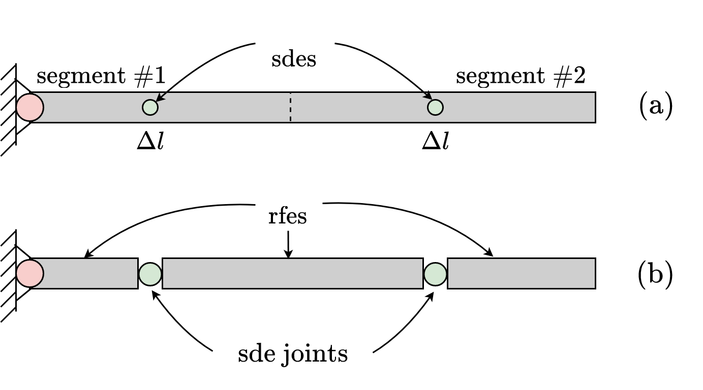
1. Primary division: dividing the deformable object of length \(L\) into relatively simple elements with finite dimension \(\Delta l\) and concentrating their spring and damping features at one point (see Figure 2a);
2. Secondary division: isolating rfes between sdes from the primary division to obtain a system of rfes connected by sdes (see Figure 2b).

After discretization, we can treat the system as a serial chain of rigid bodies and derive its dynamics using the Lagrange or the Newton-Euler methods. To illustrate the general form of the RFEM dynamics, let’s briefly go through the dynamics derivation using the Lagrange method. Let \(q = [q_a\ q_p]^T\) denote the vector of joint angles, with \(q_a\) being the active joint angle and \(q_p\) being the passive joint angles of sdes. Using generalized coordinates, we can write down the energy functions used in the Lagrangian method

Here \(n_s\) is the number of segments, \(M(q)\) is the inertia matrix, \(K\) and \(D\) are the constant diagonal stiffness and damping matrices, respectively; \(m_i\) and \(p_{C_i}\) are \(i-\)the rfes mass and the center of mass, respectively; \(g_0 = [0\ 0\ -9.81]^T\) is the gravity acceleration vector. Applying the Lagrange equations

with \(\mathcal{L} = K - P\) being the Lagrangian, we get the final expression for the RFEM dynamics:

Comparing the final expression for RFEM dynamics to classical rigid-body manipulator dynamics, we see two new terms: \(Kq\) representing linear spring forces and \(D\dot q\) representing linear damper forces. Despite these new terms, the difference between RFEM dynamics and classical rigid-body dynamics is minor. Therefore, we can adapt existing efficient rigid-body algorithms to compute RFEM dynamics, and there is no need to implement new software.

For simulation and control we often need state-space models. To convert the RFEM dynamics (*) to state-space form, we define a state vector \(x=[q\ \dot q]^T\) and input \(u:= \tau\):

Parameters of rfes and sdes

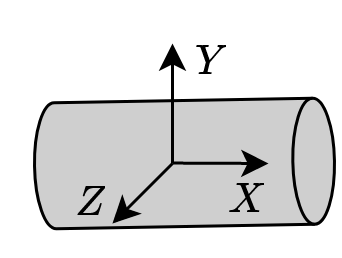
The mass \(m_i\), first moment of inertia \(h=m_i p_{C_i}\), and second moments of inertia \(I_i\) expressed in the frame located at the center of mass of an rfe are the fundamental parameters of the rfe. In the case of homogenous (constant density \(\rho\)) objects with constant cross-section, these inertial parameters can be calculated using standard formulas. For our toy example — for a homogenous cylicrical shape rfe with length \(l\) and diameter \(d\) (as in Figure 3) — formulae are:

However, for deformable objects with varying cross-sections and more complex shapes, CAD software is required.

Linear spring and damping parameters are the basic parameters of the sde. The stiffness \(k_i\) of the spring is a three-dimensional diagonal matrix, while for the planar case, \(k_i\) is a scalar. Similarly, the damping parameters \(d_i\) also follow the same rule.

The coefficients of stiffness and damping of the sde are based on the elasticity features of a beam segment with length \(\Delta l\), such that the real segment of the beam will deform in the same way and with the same velocities of deformation as the equivalent sde under the same load. For homogenous materials of a specific constant cross-section, there are readily available formulas to calculate these coefficients. For our toy example, formulae are

where \(G\) is the shear modulus and \(E\) is Young’s modulus. However, for more complex shapes, CAD software must be utilized.

Tutorial: implementing the RFEM with Pinocchio to simulate flexible pendulum

The tutorial leverages Pinocchio, an amazing tool for robot dynamics! Developed by Justin Carpentier, Pinocchio implements Roy Featherstone algorithms in C++, making it incredibly efficient. But that’s not all - it’s also been extended with new algorithms for computing derivatives of dynamics algorithms, constrained dynamics, and more. The best part? You can generate dynamics algorithms as a Casadi function and use them in optimal controller design.

In this tutorial (link to code), we will define the setup using URDF, which supports geometry and inertial parameters but unfortunately doesn’t support joint elasticity. Therefore, we will use an additional .yaml file to define sde parameters. To modify the geometry and inertial parameters of the RFEM, you will need to manually update the URDF files. But it’s easy to modify sde parameters (which is the most fun part) from the rod_params.py file by changing the \(G\) and \(E\) values. You can even use this file to compute the inertial parameters for a desired cylindrical rod.

Computing dynamics

Now, to simulate the flexible pendulum, we need to compute the forward dynamics of the RFEM model. The most efficient algorithm to use for this is articulated rigid body (ABA). Unfortunately, ABA in Pinocchio doesn’t support flexible joints (sdes) by default. But fear not, we can restructure the RFEM dynamics equation to treat sde torques as an input to the system

where \(\tilde \tau = B \tau - K q - D \dot{q}\). This is possible because sde joints are virtual and are not actuated.

To implement the flexible pendulum model, I have created a FlexiblePendulum class in the flexible_pendulum.py module. This class takes the number of segments as input and builds the model in its __init__ method. Additionally, the class contains several other useful methods:

def elasticity_torques(self, q: np.ndarray, dq: np.ndarray):
    """ Computes torques due to elastic elements in the
    joints: spring-damper elements
    NOTE the first joint -- active joint -- doesn't
         have spring-damper element in it

    :param q: joint positions
    :param dq: joint velocities

    :return: torques 
    """
    return -self.K @ q - self.D @ dq

def forward_dynamics(self, q:np.ndarray, dq:np.ndarray, tau_a:np.ndarray):
    """ Computes forward dynamics

    :param q: joint positions
    :param dq: joint velocities
    :param tau_a: active joints torque

    :return: ddq -- aceelerations of all joints, active and passive 
    """
    tau = self.B @ tau_a + self.elasticity_torques(q, dq)

    return pin.aba(self.model, self.data, q, dq, tau).reshape(-1, 1)

def ode(self, x: np.ndarray, u: np.ndarray):
    """ Computes ode of the robot

    :param x: robot state
    :param u: active joint torque

    :return: x_dot
    """
    q, dq = np.split(x, 2)
    return np.vstack((dq, self.forward_dynamics(q, dq, u)))

Integrating RFEM dynamics

It’s important to note that RFE dynamics can be quite stiff, and using fixed-step integrators can result in divergence if the step size is too large. To avoid this problem, I have opted to use a variable step Runge-Kutta integrator from the scipy.integrate package in this tutorial.

In order to simulate the flexible pendulum system, I have implemented a simulate_flexible_pendulum function in the simulation.py module. Additionally, to incorporate a controller into the simulation, I created a controllers.py file which contains an abstract BaseController class. To provide concrete implementations of controllers, I created a DummyController class that always returns zero torque, and a PDController that implements a proportional-derivative controller. By inheriting from the BaseController class, it is easy to create new controllers as needed.

By using the variable step integrator and implementing controllers, we can now simulate the flexible pendulum system and explore its behavior under various conditions.

Visualization

Pinocchio provides several options for visualizing robots. In order to visualize the motion of the flexible pendulum system, I have implemented visualize_elastic_pendulum function in the visualization.py module which can use either the Meshcat or Panda3d visualizers of Pinocchio.

Some simulation results

When using RFEM to model deformable objects, the accuracy is greatly influenced by the level of discretization. Specifically, the approximation of natural frequency of the continuum material is impacted. As with any discretization method, increasing the level of discretization improves the accuracy of the approximation.

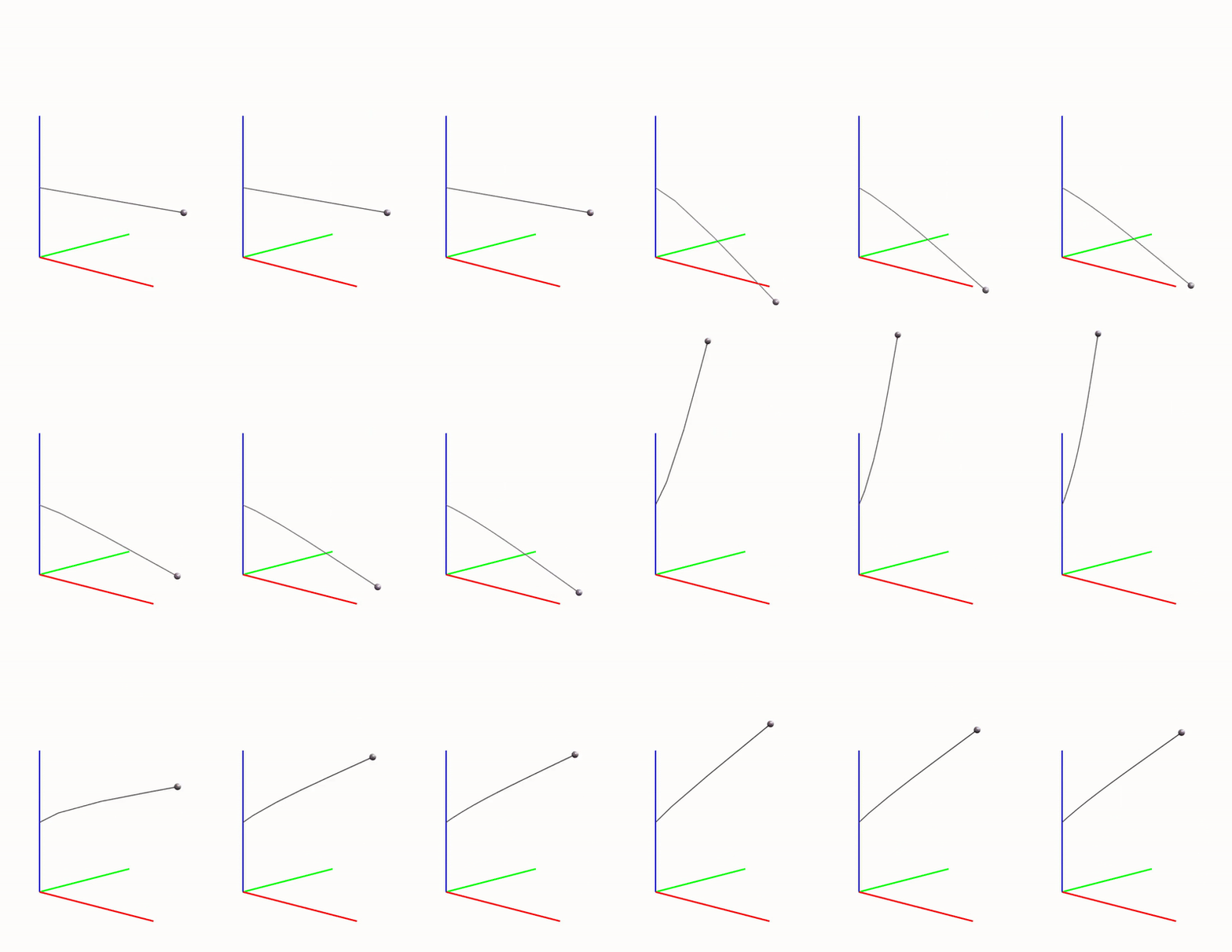
To demonstrate this visually, let’s analyze the motion of a pendulum using three different discretizations: models with 3, 5, and 10 segments. If you’re interested in a more quantitative analysis, please refer to preprint of our paper or the RFEM book.

We’ll use a PD controller with a zero reference for the active angle \(q_a^r = 0\) rad for 2.5 seconds, then change the reference to \(q_a^r = \pi/4\) rad for the next 2.5 seconds. The GIF below visualizes the motion of all three models. While there may be small synchronization errors, there is a noticeable difference: the model with 3 segments behaves differently compared to the models with 5 and 10 segments, which move similarly.

Final comments and recommendations

If you clone the code and run main.py with a 10-segment discretization, you’ll notice that the integration is quite slow. This is due to two reasons: (i) the scipy implementation of RK45 is inefficient and (ii) the state-space dimension is simply too large. In the past, I used the CVODES integrator, which resulted in a much faster simulation time. Alternatively, fixed-step implicit integrators are a good choice for optimization-based control.

Overall, the RFEM method is a straightforward way to model deformable objects, and it can make use of existing tools for modeling rigid robots. However, one of its main limitations is that it requires very fine discretization to accurately model deformable objects, which can result in slow computation times.