Introduction

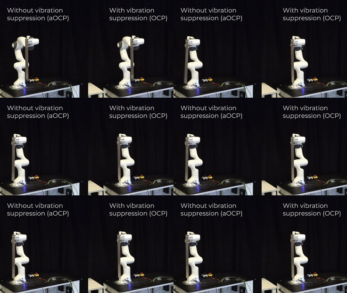
Imagine you want to dynamically manipulate a flexible object such as a beam with a robot arm. If you naively plan a trajectory and excute it, you will end up with large vibraions, as shown below.

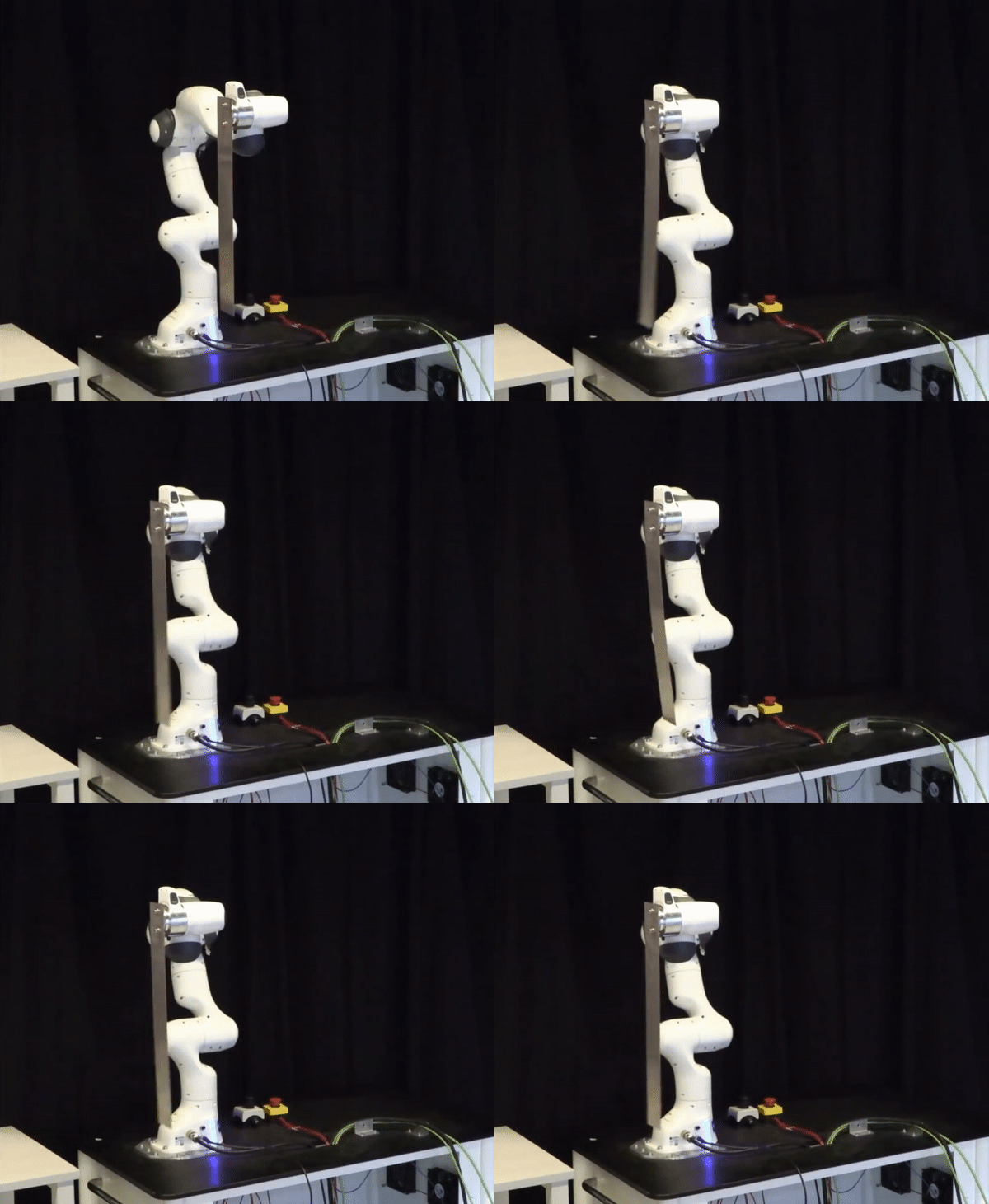
Vibrations of a beam in case of naive trajectory planning

Existing solutions for addressing the vibrations

use expensive sensors such as force-torque sensors;
require specialized grippers such as vacuum grippers;
exploit complicated dynamic models of the whole system.

Method

We propose a method for vibration-free manipulation of flexible beams that does not require any exteroceptive sensor.

Figure 1. The proposed method for vibration-free beam handling

Given a task specification – such as initial configuration of the robot \(q\) and and a final position of the beam’s tip – the method utilizes a simple dynamic model of the beam and plans a trajectory in the joint space of the robot: \(q(t),\ \dot q(t)\) and \(\ddot q(t)\)). Subsequently, the optimized trajectory is executed by a robot and results in almost vibration-free task execution.

Modeling

For modeling the robot arm we assume that the internal joint controller can accurately track the joint reference trajectories. Under this assumption the robots model is

\[\ddot q = u\]

where \(u\) are the control inputs: commanded joint accelerations.

To model the beam, we approximate it by a simple pendulum connected to the end-effector of an arm through passive revolute joint with stiffness \(k\) and damping \(c\)

\[\begin{align*} \ddot \theta = &- 2\textcolor{red}{\zeta \omega_n} \dot \theta - \textcolor{red}{\omega_n}^2 \theta + \frac{1}{\textcolor{red}{l}}{ i}^\top \frac{d R_z(\theta)}{d \theta}^\top R_b^\top ( g - \ddot{ p}_{b}) \nonumber \\ & - { i}^\top \frac{d R_z(\theta)}{d \theta}^\top R_b^\top S(\dot{ \omega}_b) R_b R_z(\theta) { i} \label{eq:pend_dynamics} \\ & + { i}^\top\frac{d R_z(\theta)}{d \theta}^\top R_{b}^\top S( \omega_b)^\top S( \omega_b) R_{b} R_z(\theta){ i} \nonumber. \end{align*}\]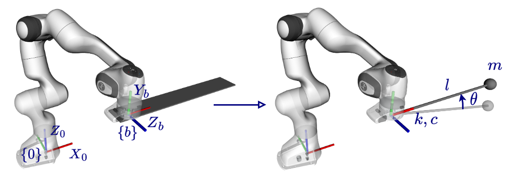

Figure 2. Illustration of approximating a beam attached to the end-effector of a robot arm with a simple pendulum attached to the end-effector by means of a passive revolute joint with stiffness \(k\) and damping \(c\).

Parameter esstimation

Although the model has a few parameters, estimating them is not straightforward as there are no accurate wrench or acceleration measurements to fit the parameters of the model using classical system identification methods. Instead, we need to infer the parameters from noisy external wrench estimate provided by the robot manufacturer. To this end, we designed dedicated experiments, as shown in the Figure ?, based on the model properties to estimate parameters using only peaks of the oscillations.

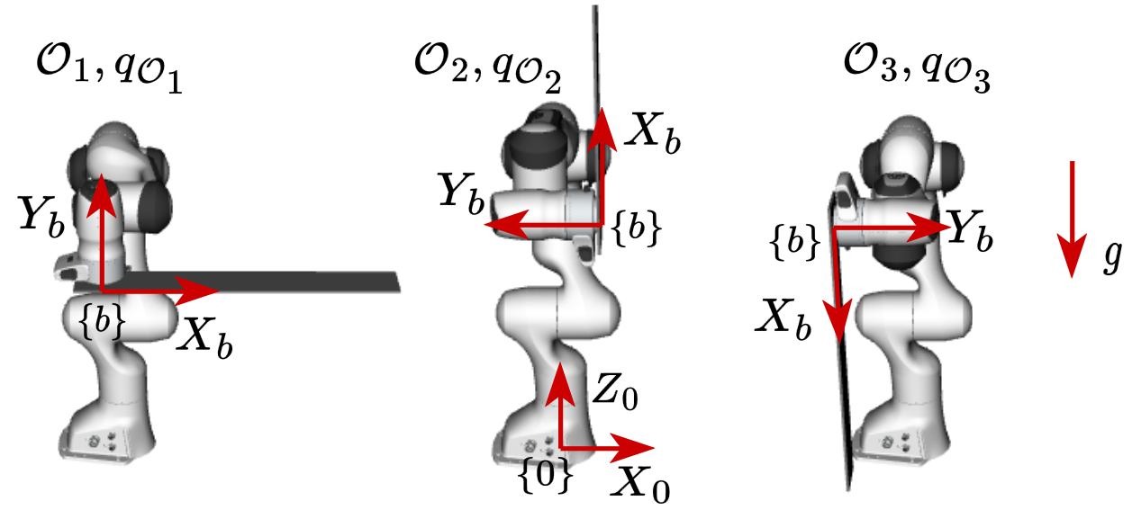
Figure 3. Orientations of the robot used in parameter estimation experiments. In all cases the motion of the robot was along local \(Y_b\) axis by 15, 25 and 25cms.

Estimation results show that linear spring model is an adequate assumption, while linear damper is an oversimplification.

Figure 4. Box plots of the estimated periods of damped oscillations and log decrement for each orientation \(\mathcal{O}_i,\ i=\{1,2,3\}\). Data for each orientation consisted of three experiments, each repeated six times.

Trajectory Optimization

To manipulate the beam we formulate the optimal control problem (OCP) in the joint space because it is easier to impose constraints and allows to achieve faster trajectories. To make trajectories smooth, the time derivative of inputs (joint accelerations) were penalized.

\[\begin{align*} \underset{x, u}{\text{min}} &\int_{0}^{t_f} \left(||x-x_0||_{W_x} + || u||_{W_u} + \rho ||\dot{ u}||_2 \right) dt \\ \text{s.t.}\ &\dot{ x} = f( x, u) \\ &x(0) = [ q_0^\top\ \theta_{0}\ 0^\top]^\top,\ u(0) = 0 \\ & p_{b}\left( q(t_f)\right) = p_{b, t_f},\ \dot{ q}(t_f) = 0,\ u(t_f) = 0 \\ &\theta(t_f) = \theta_{t_f},\ \dot \theta(t_f) = 0 \\ & e_O\left( R_{b}\left( q(t_f)\right), R_{b, t_f}\right) = 0_{3\times 1} \\ & x \in \mathcal{X},\ u \in \mathcal{U}, \ \dot{ u} \in \mathcal{J} \end{align*}\]

The OCP was cast as nonlinear program (NLP) following the multiple-shooting method and solve the NLP using IPOPT.

Results

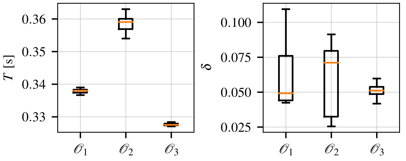
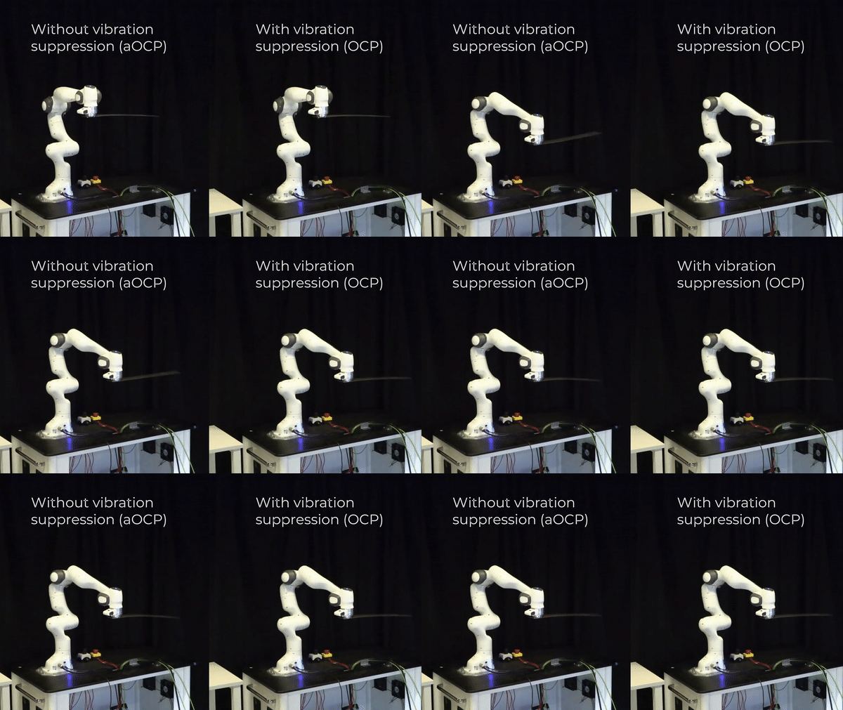
To test the proposed method, we performed three tasks: 1D motion (T1), 2D motion (T2) and 6D motion (T3).

T1: Starting from \(q_0 = q_{\mathcal{O}_3}\), as in Figure 3, move the end-effector by \(-0.20\ \mathrm{m}\) along the \(X_0-\)axis.

T2: Starting from \(q_0 = q_{\mathcal{O}_1}\), as in Figure 3, move the end-effector by \([0.20\ 0\ -0.20]^\top\ \mathrm{m}\) relative to \(\{0\}\).

T3: Starting from \(q_0 = q_{\mathcal{O}_2}\), as in Figure 3, move the end-effector by \([0.20\ 0\ -0.20]^\top\ \mathrm{m}\) relative to \(\{0\}\) and orient \(\{b\}\) like \(\mathcal{O}_1\) but rotated by \(90\ \mathrm{deg}\) around \(Z_0\).

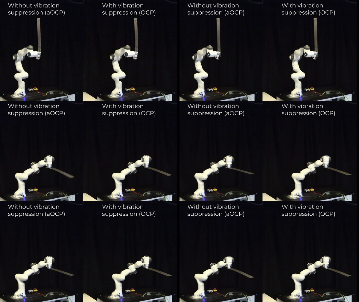
For each task we achieve similar or beter performance than zero vibrations input shaping while being significantly faster.

Conclusions

In this work, we proposed:

A model that is simple yet effectively captures the complex dynamics of the system.
An OCP for handling the beam that drastically reduces residual vibrations and allows us to trade off vibration suppression and task execution time.
Experimental validation of the proposed method and comparison with input shaping.